【Backgroud】
Sabour S, Frosst N, Hinton G E. Dynamic Routing Between Capsules[J]. NIPS2017
【环境】
-
CUDA: 9.2.148
-
Torch:1.2.0
-
OS: Ubuntu 16.04
-
HW: Nvidia Tesla P100 / Nvidia GTX 1080Ti / Nvidia RTX 2080Ti
【关于CapsNet的介绍】
见文:【CapsNet】Dynamic Routing Between Capsules
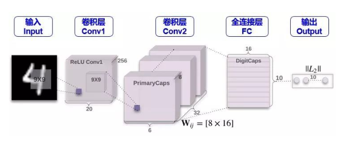
【从模型说起】

Conv1
这一步就是一个常规的卷积操作,用了 256 个 stride 为 1 的 9×9 的 filter,得到一个 20x20x256 的输出。按照原文的意思,这一步主要作用就是对图像像素做一次局部特征检测。让我们 Conv1 层的维度是如何得到的。(但为什么不一开始就用 Capsule 呢?因为 Capsule 是用来表征某个物体的“实例”,因此它更适合于表征高级的实例。如果直接用 Capsule 吸取图片的低级特征内容,不是很理想,而 CNN 却擅长抽取低级特征,因此一开始用 CNN 是合理的)
整个CapsuleNet代码实现如下:
class CapsuleNet(nn.Module):
    """Basic implementation of capsule network layer."""

    def __init__(self):
        super(CapsuleNet, self).__init__()

        # Conv2d layer
        self.conv = nn.Conv2d(1, 256, 9)
        self.relu = nn.ReLU(inplace=True)

        # Primary capsule
        self.primary_caps = PrimaryCaps(num_conv_units=32,
                                        in_channels=256,
                                        out_channels=8,
                                        kernel_size=9,
                                        stride=2)

        # Digit capsule
        self.digit_caps = DigitCaps(in_dim=8,
                                    in_caps=32 * 6 * 6,
                                    out_caps=10,
                                    out_dim=16,
                                    num_routing=3)

        # Reconstruction layer
        self.decoder = nn.Sequential(
            nn.Linear(16 * 10, 512),
            nn.ReLU(inplace=True),
            nn.Linear(512, 1024),
            nn.ReLU(inplace=True),
            nn.Linear(1024, 784),
            nn.Sigmoid())

    def forward(self, x):
        out = self.relu(self.conv(x))
        out = self.primary_caps(out)
        out = self.digit_caps(out)

        # Shape of logits: (batch_size, out_capsules)
        logits = torch.norm(out, dim=-1)
        pred = torch.eye(10).to(device).index_select(dim=0, index=torch.argmax(logits, dim=1))

        # Reconstruction
        batch_size = out.shape[0]
        reconstruction = self.decoder((out * pred.unsqueeze(2)).contiguous().view(batch_size, -1))

        return logits, reconstruction
PrimaryCaps:
Conv2 层才是开始含有 Capsule。如果按照普通 CNN 里面的做法,用了 32 个 stride 为 2 的 9x9x256 的 filter,也只能得到 6x6x32 的输出,算法如下:
但是从上图和 Hinton 的论文发现,Conv2 层的维度是 6x6x8x32。这个 8怎么来的?它又代表着什么含义?个人理解是用 32 个 stride 为 2 的 9x9x256 的filter做了 8次卷积操作,而且
-
在 CNN 中,维度为 6x6x1x32 的层里有 6x6x32 元素,每个元素是一个标量
-
在 Capsule 中,维度为 6x6x8x32 的层里有 6x6x32 元素,每个元素是一个 1×8的向量,既 capsule
Conv2 层的输出在论文中称为 Primary Capsule,简称 PrimaryCaps,主要储存低级别特征的向量。
Primary Capsule模型定义代码如下:
class PrimaryCaps(nn.Module):
    """Primary capsule layer."""

    def __init__(self, num_conv_units, in_channels, out_channels, kernel_size, stride):
        super(PrimaryCaps, self).__init__()

        # Each conv unit stands for a single capsule.
        self.conv = nn.Conv2d(in_channels=in_channels,
                              out_channels=out_channels * num_conv_units,
                              kernel_size=kernel_size,
                              stride=stride)
        self.out_channels = out_channels

    def forward(self, x):
        # Shape of x: (batch_size, in_channels, height, weight)
        # Shape of out: out_capsules * (batch_size, out_channels, height, weight)
        out = self.conv(x)
        # Flatten out: (batch_size, out_capsules * height * weight, out_channels)
        batch_size = out.shape[0]
        return squash(out.contiguous().view(batch_size, -1, self.out_channels), dim=-1)
DigitCaps:
下一层就是存储高级别特征的向量,在本例中就是数字,FC 层的输出在论文中称为 Digit Capsule,简称 DigitCaps。PrimaryCaps 和 DigitCaps 是全连接的,但不是像传统神经网络标量和标量相连,而是向量与向量相连。
PrimaryCaps 里面有 6x6x32 元素,每个元素是一个 1×8的向量,而 DigitCaps 有 10 个元素 (因为有 10 个数字),每个元素是一个 1×16的向量。为了让 1×8向量与 1×16向量全连接,需要 6x6x32 个 8×16的矩阵
现在 PrimaryCaps 有 6x6x32 = 1152 个 VN,而 DigitCaps 有 10 个 VN,那么 I = 1,2, …, 1152, j = 0,1, …, 9。再用小节 2.4 讲的动态路由算法迭代 3 次计算 cij并输出 10 个 vj。
DigitCaps代码如下:
class DigitCaps(nn.Module):
    """Digit capsule layer."""

    def __init__(self, in_dim, in_caps, out_caps, out_dim, num_routing):
        """
        Initialize the layer.
        Args:
            in_dim:       Dimensionality of each capsule vector.
            in_caps:      Number of input capsules if digits layer.
            out_caps:     Number of capsules in the capsule layer
            out_dim:      Dimensionality, of the output capsule vector.
            num_routing:   Number of iterations during routing algorithm
        """
        super(DigitCaps, self).__init__()
        self.in_dim = in_dim
        self.in_caps = in_caps
        self.out_caps = out_caps
        self.out_dim = out_dim
        self.num_routing = num_routing
        self.device = device
        self.W = nn.Parameter(0.01 * torch.randn(1, out_caps, in_caps, out_dim, in_dim),
                              requires_grad=True)

    def forward(self, x):
        batch_size = x.size(0)
        # (batch_size, in_caps, in_dim) -> (batch_size, 1, in_caps, in_dim, 1)
        x = x.unsqueeze(1).unsqueeze(4)
        # W @ x =
        # (1, out_caps, in_caps, out_dim, in_dim) @ (batch_size, 1, in_caps, in_dim, 1) =
        # (batch_size, out_caps, in_caps, out_dims, 1)
        u_hat = torch.matmul(self.W, x)
        # (batch_size, out_caps, in_caps, out_dim)
        u_hat = u_hat.squeeze(-1)
        # detach u_hat during routing iterations to prevent gradients from flowing
        temp_u_hat = u_hat.detach()

        b = torch.zeros(batch_size, self.out_caps, self.in_caps, 1).to(self.device)

        for route_iter in range(self.num_routing - 1):
            # (batch_size, out_caps, in_caps, 1) -> Softmax along out_caps
            c = b.softmax(dim=1)

            # element-wise multiplication
            # (batch_size, out_caps, in_caps, 1) * (batch_size, in_caps, out_caps, out_dim) ->
            # (batch_size, out_caps, in_caps, out_dim) sum across in_caps ->
            # (batch_size, out_caps, out_dim)
            s = (c * temp_u_hat).sum(dim=2)
            # apply "squashing" non-linearity along out_dim
            v = squash(s)
            # dot product agreement between the current output vj and the prediction uj|i
            # (batch_size, out_caps, in_caps, out_dim) @ (batch_size, out_caps, out_dim, 1)
            # -> (batch_size, out_caps, in_caps, 1)
            uv = torch.matmul(temp_u_hat, v.unsqueeze(-1))
            b += uv

        # last iteration is done on the original u_hat, without the routing weights update
        c = b.softmax(dim=1)
        s = (c * u_hat).sum(dim=2)
        # apply "squashing" non-linearity along out_dim
        v = squash(s)

        return v
【损失函数】
\( L_k = T_k \max (0, m^+ – ||V_k||)^2 + \lambda (1-T_k) \max(0, ||V_k|| – m^-)^2\)
下标\(k\)是分类
\( T_k \)是分类的指示函数 (k 类存在为 1,不存在为 0)
\( m^+\)为上界,惩罚假阳性 (false positive) ,即预测 k 类存在但真实不存在,识别出来但错了
\( m^-\)为下界,惩罚假阴性 (false negative) ,即预测 k 类不存在但真实存在,没识别出来
\( \lambda\)是比例系数,调整两者比重
总的损失是各个样例损失之和。论文中 \( m^+ = 0.9, m^- = 0.1, \lambda = 0.5\),用大白话说就是
如果 k 类存在,\( ||V_k||\)不会小于 0.9
如果 k 类不存在,\( ||V_k||\) 不会大于 0.1
惩罚假阳性的重要性大概是惩罚假阴性的重要性的 2 倍
损失函数定义如下:
class CapsuleLoss(nn.Module):
    """Combine margin loss & reconstruction loss of capsule network."""

    def __init__(self, upper_bound=0.9, lower_bound=0.1, lmda=0.5):
        super(CapsuleLoss, self).__init__()
        self.upper = upper_bound
        self.lower = lower_bound
        self.lmda = lmda
        self.reconstruction_loss_scalar = 5e-4
        self.mse = nn.MSELoss(reduction='sum')

    def forward(self, images, labels, logits, reconstructions):
        # Shape of left / right / labels: (batch_size, num_classes)
        left = (self.upper - logits).relu() ** 2  # True negative
        right = (logits - self.lower).relu() ** 2  # False positive
        margin_loss = torch.sum(labels * left) + self.lmda * torch.sum((1 - labels) * right)

        # Reconstruction loss
        reconstruction_loss = self.mse(reconstructions.contiguous().view(images.shape), images)

        # Combine two losses
        return margin_loss + self.reconstruction_loss_scalar * reconstruction_loss
【训练步骤】
话不多说,代码奉上:
def train(model, train_loader, test_loader, args, device):
    criterion = CapsuleLoss()
    optimizer = Adam(model.parameters(), lr=args.lr) # from torch.optim import Adam, lr_scheduler
    scheduler = lr_scheduler.ExponentialLR(optimizer, gamma=args.weight_delay)
    model.train()
    for epoch in range(args.epochs):
        correct, total, total_loss = 0, 0, 0.
        for x, y in tqdm(train_loader): #tqdm is the funtion of proccessing bar
            optimizer.zero_grad()
            x = x.to(device)
            y = torch.eye(10).index_select(dim = 0, index = y).to(device)
            y_pred, x_recon = model(x)

            loss = criterion(x, y, y_pred, x_recon)
            correct += torch.sum(
                torch.argmax(y_pred, dim=1) == torch.argmax(y, dim=1)
            ).item()
            total += len(y)
            accuracy = correct / total
            total_loss += loss
            loss.backward()
            optimizer.step()
        scheduler.step(epoch)
        val_loss, val_accuracy = evaluate(model=model, test_loader=test_loader, device=device) #evaluate funtion will introduction below
        print('Epoch: %d, train_accuracy: %.2f , val_loss: %.2f , val_accuracy: %.2f ' % ((epoch + 1), accuracy * 100, val_loss * 100, val_accuracy * 100))
【一些补充工具】
def load_mnist(path='./datas', download=True, batch_size=128, shift_pixels=2):
    kwargs = {
        'num_workers' : 4,
        'pin_memory' : True
    }
    transform = transforms.Compose([
        # shift by 2 pixels in either direction with zero padding.
        transforms.RandomCrop(28, padding=2),
        transforms.ToTensor(),
        transforms.Normalize((0.1307,), (0.3081,))
    ])
    train_loader = torch.utils.data.DataLoader(
        datasets.MNIST(root=path, download=download, train=True, transform=transform),
        batch_size=batch_size,
        shuffle=True, **kwargs)
    test_loader = torch.utils.data.DataLoader(
        datasets.MNIST(root=path, download=download, train=False, transform=transform),
        batch_size=batch_size,
        shuffle=True, **kwargs)
    return train_loader, test_loader

def evaluate(model, test_loader, device):
    model.eval()
    correct, total = 0, 0
    for images, labels in test_loader:
        # Add channels = 1
        images = images.to(device)
        # Categogrical encoding
        labels = torch.eye(10).index_select(dim=0, index=labels).to(device)
        logits, reconstructions = model(images)
        pred_labels = torch.argmax(logits, dim=1)
        correct += torch.sum(pred_labels == torch.argmax(labels, dim=1)).item()
        total += len(labels)

    return 1 - correct / total, correct / total

if __name__ == '__main__':
    args, option = getParams()
    device = torch.device('cuda' if torch.cuda.is_available() else 'cpu')
    model = CapsuleNet()
    model = model.to(device)
    print(model)
    train_loader, test_loader = load_mnist(batch_size=args.batch_size)
    train(model, train_loader, test_loader, args, device)
【参考文献】
-
Sabour S, Frosst N, Hinton G E. Dynamic Routing Between Capsules[J]. NIPS2017
【附Code GitHub】
传送点:Click Me
环境Docker Hub: Click Me
【实验截图】
